A Tour of R’s Programming ‘Dialects’

code
Author

Daniel B. Cooper (daniel.cooper@ky.gov)

Published

June 6, 2025

Modified

August 21, 2025

Introduction 🗣️

In the R world, you’ll often hear about different “dialects” or ways of writing code. While they all get you to the same destination, the journey looks quite different. Today, we’ll explore three of the most popular approaches for data manipulation:

  • Base R: The original, built-in syntax of R.
  • The Tidyverse: An opinionated collection of packages designed for data science that share a common philosophy.
  • data.table: A package optimized for speed and memory efficiency, known for its concise syntax.

We’ll use the built-in mtcars dataset for all our examples to perform a simple task: Find the average miles per gallon (mpg) and horsepower (hp) for all 8-cylinder (cyl) cars.

# load data explicitly
mtcars <- datasets::mtcars

# Take a peek at the data
head(mtcars)
                   mpg cyl disp  hp drat    wt  qsec vs am gear carb
Mazda RX4         21.0   6  160 110 3.90 2.620 16.46  0  1    4    4
Mazda RX4 Wag     21.0   6  160 110 3.90 2.875 17.02  0  1    4    4
Datsun 710        22.8   4  108  93 3.85 2.320 18.61  1  1    4    1
Hornet 4 Drive    21.4   6  258 110 3.08 3.215 19.44  1  0    3    1
Hornet Sportabout 18.7   8  360 175 3.15 3.440 17.02  0  0    3    2
Valiant           18.1   6  225 105 2.76 3.460 20.22  1  0    3    1

1. Base R 🧱

Base R is the foundation of the R language. It requires no external packages and is incredibly powerful and flexible. The syntax often involves using brackets [ for subsetting and the $ operator to access columns (data frame variables).

Data Manipulation with Base R

Here, we first create a logical vector is_8_cyl to identify the rows we want. We then use that vector to subset the data frame and finally apply the mean() function to the columns of interest using lapply().

# First, create a logical index for 8-cylinder cars
is_8_cyl <- mtcars$cyl == 8

# Subset the data frame using the logical index
eight_cyl_cars <- mtcars[is_8_cyl, ]

# Calculate the mean for the desired columns
avg_stats_base <- lapply(eight_cyl_cars[, c("mpg", "hp")], mean)

print(avg_stats_base)
$mpg
[1] 15.1

$hp
[1] 209.2143

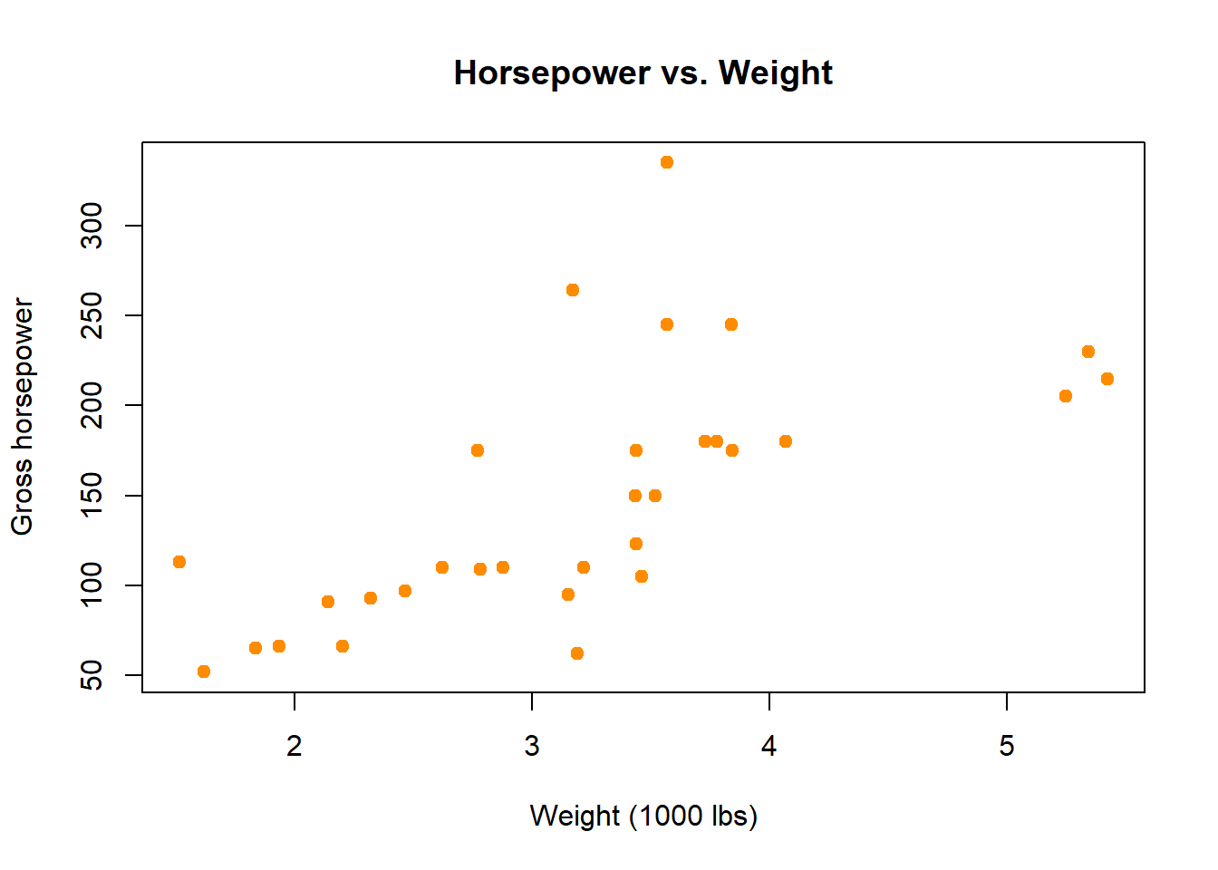
Plotting with Base R

Base R graphics are excellent for creating quick, standard plots. The plot() function is a workhorse for scatter plots.

plot(mtcars$wt, mtcars$hp,
     main = "Horsepower vs. Weight",
     xlab = "Weight (1000 lbs)",
     ylab = "Gross horsepower",
     pch = 19,
     col = "darkorange")

Base R scatter plot of horsepower vs. weight.

2. The Tidyverse ✨

The Tidyverse is a collection of packages (like {dplyr} and {ggplot2}) designed to make data science more intuitive. It emphasizes readable code and uses the pipe operator (|>) to chain functions together into a clean, sequential workflow.

Data Manipulation with the Tidyverse

The same task in the Tidyverse is a sequence of readable “verbs.” We take the mtcars data, convert the data frame to a “tibble” (an opinionated data frame that changes print and other function methods) using as_tibble(), filter() it to keep only the 8-cylinder cars, and then summarize() by calculating the mean() for our columns.

# We need to load the library first
library(dplyr)
Warning: package 'dplyr' was built under R version 4.4.3

Attaching package: 'dplyr'
The following objects are masked from 'package:stats':

    filter, lag
The following objects are masked from 'package:base':

    intersect, setdiff, setequal, union
library(tibble)

mtcars_tibble <- as_tibble(mtcars)

print(mtcars)
                     mpg cyl  disp  hp drat    wt  qsec vs am gear carb
Mazda RX4           21.0   6 160.0 110 3.90 2.620 16.46  0  1    4    4
Mazda RX4 Wag       21.0   6 160.0 110 3.90 2.875 17.02  0  1    4    4
Datsun 710          22.8   4 108.0  93 3.85 2.320 18.61  1  1    4    1
Hornet 4 Drive      21.4   6 258.0 110 3.08 3.215 19.44  1  0    3    1
Hornet Sportabout   18.7   8 360.0 175 3.15 3.440 17.02  0  0    3    2
Valiant             18.1   6 225.0 105 2.76 3.460 20.22  1  0    3    1
Duster 360          14.3   8 360.0 245 3.21 3.570 15.84  0  0    3    4
Merc 240D           24.4   4 146.7  62 3.69 3.190 20.00  1  0    4    2
Merc 230            22.8   4 140.8  95 3.92 3.150 22.90  1  0    4    2
Merc 280            19.2   6 167.6 123 3.92 3.440 18.30  1  0    4    4
Merc 280C           17.8   6 167.6 123 3.92 3.440 18.90  1  0    4    4
Merc 450SE          16.4   8 275.8 180 3.07 4.070 17.40  0  0    3    3
Merc 450SL          17.3   8 275.8 180 3.07 3.730 17.60  0  0    3    3
Merc 450SLC         15.2   8 275.8 180 3.07 3.780 18.00  0  0    3    3
Cadillac Fleetwood  10.4   8 472.0 205 2.93 5.250 17.98  0  0    3    4
Lincoln Continental 10.4   8 460.0 215 3.00 5.424 17.82  0  0    3    4
Chrysler Imperial   14.7   8 440.0 230 3.23 5.345 17.42  0  0    3    4
Fiat 128            32.4   4  78.7  66 4.08 2.200 19.47  1  1    4    1
Honda Civic         30.4   4  75.7  52 4.93 1.615 18.52  1  1    4    2
Toyota Corolla      33.9   4  71.1  65 4.22 1.835 19.90  1  1    4    1
Toyota Corona       21.5   4 120.1  97 3.70 2.465 20.01  1  0    3    1
Dodge Challenger    15.5   8 318.0 150 2.76 3.520 16.87  0  0    3    2
AMC Javelin         15.2   8 304.0 150 3.15 3.435 17.30  0  0    3    2
Camaro Z28          13.3   8 350.0 245 3.73 3.840 15.41  0  0    3    4
Pontiac Firebird    19.2   8 400.0 175 3.08 3.845 17.05  0  0    3    2
Fiat X1-9           27.3   4  79.0  66 4.08 1.935 18.90  1  1    4    1
Porsche 914-2       26.0   4 120.3  91 4.43 2.140 16.70  0  1    5    2
Lotus Europa        30.4   4  95.1 113 3.77 1.513 16.90  1  1    5    2
Ford Pantera L      15.8   8 351.0 264 4.22 3.170 14.50  0  1    5    4
Ferrari Dino        19.7   6 145.0 175 3.62 2.770 15.50  0  1    5    6
Maserati Bora       15.0   8 301.0 335 3.54 3.570 14.60  0  1    5    8
Volvo 142E          21.4   4 121.0 109 4.11 2.780 18.60  1  1    4    2
print(mtcars_tibble)
# A tibble: 32 × 11
     mpg   cyl  disp    hp  drat    wt  qsec    vs    am  gear  carb
   <dbl> <dbl> <dbl> <dbl> <dbl> <dbl> <dbl> <dbl> <dbl> <dbl> <dbl>
 1  21       6  160    110  3.9   2.62  16.5     0     1     4     4
 2  21       6  160    110  3.9   2.88  17.0     0     1     4     4
 3  22.8     4  108     93  3.85  2.32  18.6     1     1     4     1
 4  21.4     6  258    110  3.08  3.22  19.4     1     0     3     1
 5  18.7     8  360    175  3.15  3.44  17.0     0     0     3     2
 6  18.1     6  225    105  2.76  3.46  20.2     1     0     3     1
 7  14.3     8  360    245  3.21  3.57  15.8     0     0     3     4
 8  24.4     4  147.    62  3.69  3.19  20       1     0     4     2
 9  22.8     4  141.    95  3.92  3.15  22.9     1     0     4     2
10  19.2     6  168.   123  3.92  3.44  18.3     1     0     4     4
# ℹ 22 more rows
avg_stats_tidy <- mtcars_tibble |>
  filter(cyl == 8) |>
  summarize(
    avg_mpg = mean(mpg),
    avg_hp = mean(hp)
  )

print(avg_stats_tidy)
# A tibble: 1 × 2
  avg_mpg avg_hp
    <dbl>  <dbl>
1    15.1   209.

Plotting with the Tidyverse

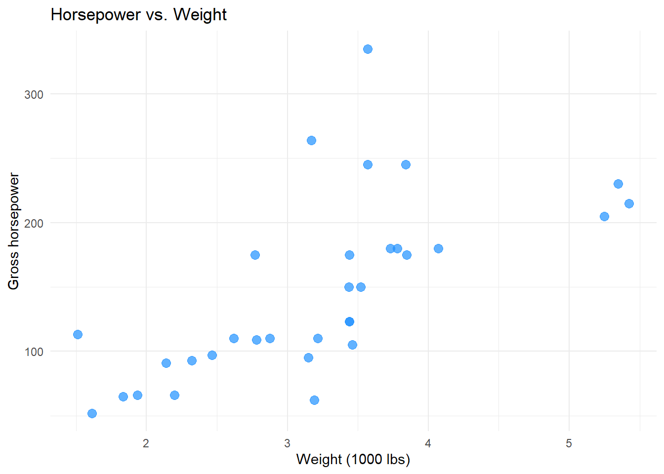
{ggplot2} is the graphics engine of the Tidyverse. It builds plots in layers, starting with ggplot() to define the data and aesthetics (aes), and then adding geometric objects (geoms) like geom_point().

library(ggplot2)

ggplot(mtcars_tibble, aes(x = wt, y = hp)) +
  geom_point(color = "dodgerblue", size = 3, alpha = 0.7) +
  labs(
    title = "Horsepower vs. Weight",
    x = "Weight (1000 lbs)",
    y = "Gross horsepower"
  ) +
  theme_minimal()

Tidyverse scatter plot of horsepower vs. weight.

3. The data.table (Tinyverse) ⚡

The {data.table} package is famous for its performance, especially with large datasets. It’s a cornerstone of the “tinyverse”—a philosophy favoring minimal dependencies and efficiency. The syntax is very concise, using the general form DT[i, j, by].

i: rows to select (where) j: columns to operate on (select or compute) by: grouping variable(s)

Data Manipulation with data.table

First, we convert the mtcars data frame into a data.table. Then, in a single, compact expression, we filter for cyl == 8 in the i slot and compute the means in the j slot.

# Load the library and convert the data
library(data.table)
Warning: package 'data.table' was built under R version 4.4.2

Attaching package: 'data.table'
The following objects are masked from 'package:dplyr':

    between, first, last
mt_dt <- as.data.table(mtcars, keep.rownames = "car")

# The i, j syntax in action
avg_stats_dt <- mt_dt[cyl == 8, .(avg_mpg = mean(mpg), avg_hp = mean(hp))]

print(avg_stats_dt)
   avg_mpg   avg_hp
     <num>    <num>
1:    15.1 209.2143

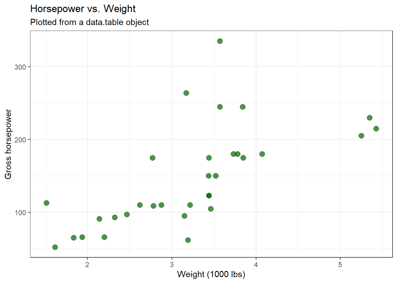
Plotting with data.table

While data.table doesn’t have its own plotting system, it works seamlessly with other plotting libraries like ggplot2 or base R’s plot().

# data.table objects are also data.frames, so ggplot2 works perfectly
ggplot(mt_dt, aes(x = wt, y = hp)) +
  geom_point(color = "darkgreen", size = 3, alpha = 0.7) +
  labs(
    title = "Horsepower vs. Weight",
    subtitle = "Plotted from a data.table object",
    x = "Weight (1000 lbs)",
    y = "Gross horsepower"
  ) +
  theme_bw()

Plotting data.table data with ggplot2.

Conclusion 🏁

Dialect Key Idea Best For…
Base R Foundational, no dependencies Scripts, understanding R’s core, minimal overhead.
Tidyverse Readability and consistency Interactive analysis, teaching, projects where clarity is key.
data.table Speed and memory efficiency Large datasets, high-performance needs, production code.

No single dialect is “best”—they are all powerful tools. The right choice depends on your specific task, the size of your data, and your personal or team’s preference. Happy coding!